STAT3002 Week 2
2.2 Adding a Predictor to SLR
Auction Data cont’. Recall the linear regression of Price vs Age :
> auc1.lm <- lm(Price ~ Age)
> summary(auc1.lm)
Call: lm(formula = Price ~ Age)
Residuals:
Min 1Q Median 3Q Max
-485.3 -192.7 30.75 157.2 541.2
Coefficients:
Value Std. Error t value Pr(>|t|)
(Intercept) -191.6576 263.8866 -0.7263 0.4733
Age 10.4791 1.7900
5.8543 0.0000
Residual standard error: 273 on 30 degrees of
freedom
Multiple R-Squared: 0.5332
F-statistic: 34.27 on 1 and 30 degrees of freedom,
the p-value is 2.096e-006
Correlation of Coefficients:
(Intercept)
Age -0.9831
The R2 = 0.5332, indicating that 53.3% of the variability in Price is explained by Age.
And the linear regression of Price vs Number of Bidders:
> summary(auc2.lm)
Call: lm(formula = Price ~ Bidders)
Residuals:
Min 1Q Median 3Q Max
-516.3
-355.3 -29.49 302.8 688.2
Coefficients:
Value Std. Error t value
Pr(>|t|)
(Intercept) 806.4049 230.6846 3.4957
0.0015
Bidders 54.6362 23.2250
2.3525 0.0254
Residual standard error: 367.2 on 30 degrees of
freedom
Multiple R-Squared: 0.1557
F-statistic: 5.534 on 1 and 30 degrees of freedom,
the p-value is 0.0254
Correlation of Coefficients:
(Intercept)
Bidders -0.9596
Are the predictors related? It is difficult to tell…
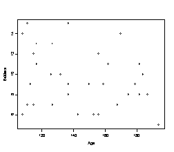
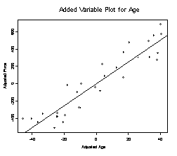
Added Variable Plot (AVP)
For this regression R2 = 0.1557, indicating that 15.6% of variability in Price is explained by Bidders. Is it reasonable to perform a regression on Price vs Age and bidders?
> auc.lm <- lm(Price
~ Age+Bidders)
> summary(auc.lm)
Call: lm(formula = Price ~
Age + Bidders)
Residuals:
Min 1Q Median 3Q
Max
-207.2 -117.8 16.49 102.7
213.5
Coefficients:
Value Std. Error t value Pr(>|t|)
(Intercept)
-1336.7221 173.3561 -7.7108 0.0000
Age 12.7362 0.9024
14.1140 0.0000
Bidders 85.8151 8.7058 9.8573 0.0000
Residual standard error:
133.1 on 29 degrees of freedom
Multiple R-Squared: 0.8927
F-statistic: 120.7 on 2
and 29 degrees of freedom, the p-value is 8.771e-015
Correlation of
Coefficients:
(Intercept) Age
Age -0.8759
Bidders -0.6701 0.2537
2.3 Introduction to Multiple
Regression
Squid Data. This Data was collected to study the size of squid eaten by sharks and tuna. The covariates are characteristics of the beak or mouth of the squid. They are:
- Beak length in inches
- Wing length in inches
- Width in inches
The response is the width of the squid in pounds.
Weight Beak Wing Width
1.95 1.31 1.07 0.35
2.90 1.55 1.49 0.47
0.72 0.99 0.84 0.32
0.81 0.99 0.83 0.27
1.09 1.05 0.90 0.30
1.22 1.09 0.93 0.31
1.02 1.08 0.90 0.31
1.93 1.27 1.08 0.34
0.64 0.99 0.85 0.29
2.08 1.34 1.13 0.37
1.98 1.30 1.10 0.38
1.90 1.33 1.10 0.38
8.56 1.86 1.47 0.65
4.49 1.58 1.34 0.50
8.49 1.97 1.59 0.59
6.17 1.80 1.56 0.59
7.54 1.75 1.58 0.59
6.36 1.72 1.43 0.63
7.63 1.68 1.57 0.68
7.78 1.75 1.59 0.62
10.15 2.19 1.86 0.72
6.88 1.73 1.67 0.55
Regression Analysis
All 3 predictors:
> squid.lm <- lm(Weight ~ Beak+Wing+Width)
> anova(squid.lm)
Analysis of Variance Table
Response: Weight
Terms added sequentially (first to last)
Df
Sum of Sq Mean Sq F Value
Pr(F)
Beak 1 199.1453 199.1453 399.0594 0.0000000
Wing 1 0.1267 0.1267 0.2538 0.6205103
Width 1 7.6701
7.6701 15.3698 0.0010027
Residuals 18 8.9827 0.4990
> summary(squid.lm)
Call: lm(formula = Weight ~ Beak + Wing + Width)
Residuals:
Min 1Q
Median 3Q Max
-1.421
-0.5198 0.09608 0.4467 0.9206
Coefficients:
Value Std. Error t value
Pr(>|t|)
(Intercept) -6.7916 0.7801 -8.7059
0.0000
Beak 4.1860 2.0355
2.0564 0.0545
Wing -1.3270 2.0965
-0.6330 0.5347
Width 14.0463 3.5828
3.9204 0.0010
Residual standard error: 0.7064 on 18 degrees of
freedom
Multiple R-Squared: 0.9584
F-statistic: 138.2 on 3 and 18 degrees of freedom,
the p-value is 1.29e-012
Correlation of Coefficients:
(Intercept) Beak Wing
Beak
-0.4758
Wing
-0.0877 -0.7073
Width 0.5440 -0.4451 -0.2846
Two predictors:
>squid.lm2 <- lm(Weight ~ Beak+Wing)
> summary(squid.lm2)
Call: lm(formula = Weight
~ Beak + Wing)
Residuals:
Min 1Q Median 3Q
Max
-2.147 -0.7121 0.1499 0.6422 1.497
Coefficients:
Value Std. Error t value Pr(>|t|)
(Intercept) -8.4556 0.8675
-9.7474 0.0000
Beak 7.7377 2.4157
3.2031 0.0047
Wing 1.0125 2.6635
0.3802 0.7080
Residual standard error:
0.9362 on 19 degrees of freedom
Multiple R-Squared: 0.9229
F-statistic: 113.7 on 2
and 19 degrees of freedom, the p-value is 2.681e-011
Correlation of
Coefficients:
(Intercept) Beak
Beak -0.3109
Wing 0.0835
-0.9715
> anova(squid.lm2)
Analysis of Variance Table
Response: Weight
Terms added sequentially (first to last)
Df
Sum of Sq Mean Sq F Value
Pr(F)
Beak 1 199.1453 199.1453 227.2154 0.0000000
Wing 1 0.1267 0.1267 0.1445 0.7080468
Residuals 19
16.6528 0.8765
One Predictor:
> squid.lm1 <- lm(Weight ~ Beak)
> summary(squid.lm3)
Call: lm(formula = Weight ~ Beak)
Residuals:
Min 1Q
Median 3Q Max
-1.993
-0.7324 0.09125 0.6395 1.615
Coefficients:
Value Std. Error t value
Pr(>|t|)
(Intercept)
-8.4831 0.8457 -10.0303
0.0000
Beak 8.6299 0.5601
15.4068 0.0000
Residual standard error: 0.916 on 20 degrees of
freedom
Multiple R-Squared: 0.9223
F-statistic: 237.4 on 1 and 20 degrees of freedom,
the p-value is 1.468e-012
Correlation of Coefficients:
(Intercept)
Beak -0.973
> anova(squid.lm1)
Analysis of Variance Table
Response: Weight
Terms added sequentially (first to last)
Df
Sum of Sq Mean Sq F Value Pr(F)
Beak 1 199.1453 199.1453 237.3686 1.467826e-012
Residuals 20 16.7794 0.8390
> summary(squid.lm1)
Call: lm(formula = Weight ~ Beak)
Residuals:
Min 1Q
Median 3Q Max
-1.993
-0.7324 0.09125 0.6395 1.615
Coefficients:
Value Std. Error t value
Pr(>|t|)
(Intercept)
-8.4831 0.8457 -10.0303
0.0000
Beak 8.6299 0.5601
15.4068 0.0000
Residual standard error: 0.916 on 20 degrees of
freedom
Multiple R-Squared: 0.9223
F-statistic: 237.4 on 1 and 20 degrees of freedom,
the p-value is 1.468e-012
Correlation of Coefficients:
(Intercept)
Beak -0.973
Variables in a different Order
> squid.lm3 <- lm(Weight ~ Width+Beak+Wing)
> anova(squid.lm3)
Analysis of Variance Table
Response: Weight
Terms added sequentially (first to last)
Df
Sum of Sq Mean Sq F Value
Pr(F)
Width 1 204.1576 204.1576 409.1034 0.0000000
Beak 1 2.5845 2.5845 5.1790 0.0353166
Wing 1 0.1999 0.1999 0.4006 0.5347209
Residuals 18
8.9827 0.4990
Added Variable Plots
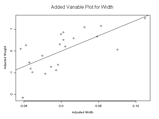
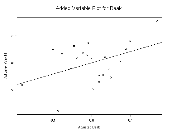
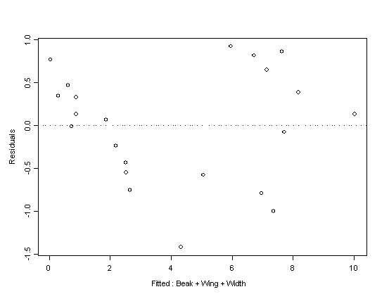
Check Assumptions!
Do the residuals look normally distributed? 