STAT3002 Week 3
1. Residuals
Hypothetical Data. The following data sets have
been artificially designed. Source:
Weisberg, 1986.
|
X |
Y |
|
X |
Y |
|
X |
Y |
|
X |
Y |
|
10 |
8.04 |
|
10 |
9.14 |
|
10 |
7.46 |
|
8 |
6.58 |
|
8 |
6.95 |
|
8 |
8.14 |
|
8 |
6.77 |
|
8 |
5.76 |
|
13 |
7.58 |
|
13 |
8.74 |
|
13 |
12.74 |
|
8 |
7.71 |
|
9 |
8.81 |
|
9 |
8.77 |
|
9 |
7.11 |
|
8 |
8.84 |
|
11 |
8.33 |
|
11 |
9.26 |
|
11 |
7.81 |
|
8 |
8.47 |
|
14 |
9.96 |
|
14 |
8.1 |
|
14 |
8.84 |
|
8 |
7.04 |
|
6 |
7.24 |
|
6 |
6.13 |
|
6 |
6.08 |
|
8 |
5.25 |
|
4 |
4.26 |
|
4 |
3.1 |
|
4 |
5.39 |
|
19 |
12.5 |
|
12 |
10.84 |
|
12 |
9.13 |
|
12 |
8.15 |
|
8 |
5.56 |
|
7 |
4.82 |
|
7 |
7.26 |
|
7 |
6.42 |
|
8 |
7.91 |
|
5 |
5.68 |
|
5 |
4.74 |
|
5 |
5.73 |
|
8 |
6.89 |
> temp1 <-
read.table("clipboard", header=T)
>
plot(temp1$X,temp1$X)
> temp1.lm <-
lm(temp1$Y ~ temp1$X)
>
abline(temp1.lm)
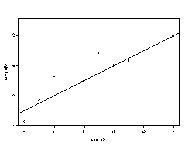
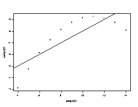
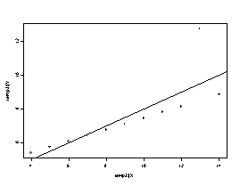
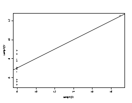
Each data set leads to the same summary regression statistics, namely
yi = 3.0 + 0.5 xi + ei, s2 =
13.75, R2 = 0.667
>
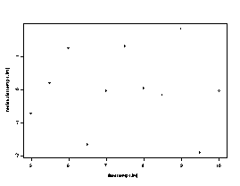
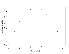
plot(fitted(temp1.lm),residuals(temp1.lm))
>
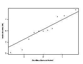
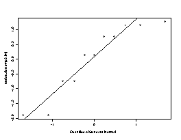
qqnorm(residuals(temp1.lm))
>
qqline(residuals(temp1.lm))
