STAT3002 Week 4
4.1 Weighted Least Squares
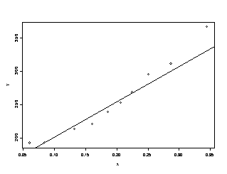
Strong Interaction of Elementary Particles. See Weisberg pages 83-88.
|
plab |
x |
y |
sd |
|
4 |
0.345 |
367 |
17 |
|
6 |
0.287 |
311 |
9 |
|
8 |
0.251 |
295 |
9 |
|
10 |
0.225 |
268 |
7 |
|
12 |
0.207 |
253 |
7 |
|
15 |
0.186 |
239 |
6 |
|
20 |
0.161 |
220 |
6 |
|
30 |
0.132 |
213 |
6 |
|
75 |
0.084 |
193 |
5 |
|
150 |
0.060 |
192 |
5 |
> attach(particles)
> w <- 1/particles$sd^2
> y1.lm <- lm(y~x,weights=w)
> summary(y1.lm)
Call: lm(formula = y ~ x, weights = w)
Residuals:
Min 1Q Median
3Q Max
-2.323 -0.8842 1.266e-006 1.39 2.335
Coefficients:
Value Std. Error
t value Pr(>|t|)
(Intercept) 148.4732 8.0786
18.3785 0.0000
x 530.8354 47.5500 11.1637
0.0000
Residual standard error: 1.657 on 8 degrees
of freedom
Multiple R-Squared: 0.9397
F-statistic: 124.6 on 1 and 8 degrees of
freedom, the p-value is 3.71e-006
Correlation of Coefficients:
(Intercept)
x -0.905
> anova(y1.lm)
Analysis of Variance Table
Response: y
Terms added sequentially (first to last)
Df Sum of Sq Mean Sq F Value Pr(F)
x 1 341.9914 341.9914 124.6287 3.710432e-006
Residuals
8 21.9526 2.7441
4.2 Testing for Lack of Fit, Variance Known
For the above data set, we have σ2=1, so we can test for lack of fit with known population variance.
For the linear regression, there is very
strong evidence, p-value = 0.005, that the linear regression is not adequate.
> pchisq(21.95,8)
[1] 0.9949907
> y2.lm <- lm(y~x+x^2,weight=w)
> summary(y2.lm)
Call: lm(formula = y ~ x + x^2, weights = w)
Residuals:
Min 1Q Median
3Q Max
-0.8993 -0.4351 0.01374 0.38 1.142
Coefficients:
Value Std. Error
t value Pr(>|t|)
(Intercept)
183.8305 6.4591 28.4609
0.0000
x 0.9709 85.3688
0.0114 0.9912
I(x^2) 1597.5047 250.5869 6.3751
0.0004
Residual standard error: 0.6788 on 7 degrees
of freedom
Multiple R-Squared: 0.9911
F-statistic: 391.4 on 2 and 7 degrees of
freedom, the p-value is 6.554e-008
Correlation of Coefficients:
(Intercept) x
x
-0.9419
I(x^2)
0.8587 -0.9736
> anova(y2.lm)
Analysis of Variance Table
Response: y
Terms added sequentially (first to last)
Df Sum of Sq Mean Sq F Value Pr(F)
x 1 341.9914 341.9914 742.1846 0.0000000230
I(x^2) 1 18.7271
18.7271 40.6413 0.0003761159
Residuals
7 3.2255 0.4608
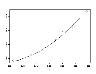
For the quadratic regression we will accept H0, p-value = 0.8629, that the quadratic regression is adequate and the linear regression is not.
> pchisq(3.23,7)
[1] 0.1370585
4.3 Testing for Lack of Fit, Variance Unknown
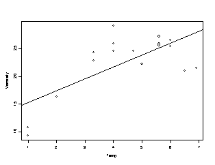
Viscosity Data Set.
Temp |
Viscosity |
Temp |
Viscosity |
|
1 |
10.84 |
5 |
22.25 |
|
1 |
9.30 |
5.6 |
27.20 |
|
2 |
16.35 |
5.6 |
25.90 |
|
3.3 |
22.88 |
5.6 |
25.61 |
|
3.3 |
24.35 |
6 |
25.45 |
|
4 |
24.56 |
6 |
26.56 |
|
4 |
25.86 |
6.5 |
21.03 |
|
4 |
29.16 |
6.9 |
21.46 |
|
4.7 |
24.59 |
|
|
> visc.lm <- lm(Viscosity~Temp)
> summary(visc.lm)
Call: lm(formula = Viscosity ~ Temp)
Residuals:
Min 1Q Median 3Q Max
-6.454 -1.616 0.5638 2.636 7.425
Coefficients:
Value Std. Error t value Pr(>|t|)
(Intercept) 13.2139 2.6649 4.9586 0.0002
Temp 2.1304 0.5645
3.7737 0.0018
Residual standard error: 4.084 on 15 degrees
of freedom
Multiple R-Squared: 0.487
F-statistic: 14.24 on 1 and 15 degrees of
freedom, the p-value is 0.001839
Correlation of Coefficients:
(Intercept)
Temp -0.9284
> anova(visc.lm)
Analysis of Variance Table
Response: Viscosity
Terms added sequentially (first to last)
Df Sum of Sq Mean Sq F
Value Pr(F)
Temp 1 237.4788 237.4788 14.2411 0.001839409
Residuals 15
250.1338 16.6756
> out.numeric <- lm(Viscosity~Temp)
> out.factor <-
lm(Viscosity~as.factor(Temp))
>
anova(out.numeric,out.factor,test="F")
Analysis of Variance Table
Response: Viscosity
Terms Resid. Df RSS Test Df Sum of Sq F Value Pr(F)
1
Temp 15 250.1338
2 as.factor(Temp) 7 15.5630 1 vs.
2 8
234.5708 13.18827 0.001388715
For the viscosity data set, the is overwhelming evidence, p-value = 0.0014, that the model is false, a more complex relationship between temperature and viscosity is needed.
4.4 Comparing Regression Lines
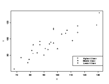
Twin Data. The data give the IQ scores of identical twins, one raised in a foster home (Y), and the other raised by natural parents (X). The data were originally used by Professor C. Burt (British J. Psychology, 1996, pp. 137-153).
> attach(twin)
> plot(X,Y,type="n")
> points(X[G1==1],Y[G1==1],pch=1)
> points(X[G2==1],Y[G2==1],pch=2)
> points(X[G3==1],Y[G3==1],pch=3)
> legend(locator(1),c("Highest Class","Middle Class","Lowest Class"),marks=c(1,2,3))
Model 1: Different slopes and intercepts.
> twin.m1 <- lm(Y~G1+G2+G3+Z1+Z2+Z3-1)
> summary(twin.m1)
Call: lm(formula = Y ~ G1 + G2 + G3 + Z1 + Z2 + Z3
- 1)
Residuals:
Min 1Q Median 3Q Max
-14.48
-5.248 -0.155 4.582 13.8
Coefficients:
Value
Std. Error t value Pr(>|t|)
G1
-1.8720 17.8083 -0.1051
0.9173
G2
0.8160 26.1092 0.0313
0.9754
G3
7.2046 16.7513 0.4301
0.6715
Z1
0.9776 0.1632 5.9902 0.0000
Z2
0.9726 0.2863 3.3973
0.0027
Z3
0.9484 0.1822 5.2061
0.0000
Residual standard error: 7.921 on 21 degrees of
freedom
Multiple R-Squared: 0.9948
F-statistic: 663.2 on 6 and 21 degrees of freedom,
the p-value is 0
Correlation of Coefficients:
G1 G2 G3
Z1 Z2
G2
0.0000
G3
0.0000 0.0000
Z1 -0.9858
0.0000 0.0000
Z2 0.0000
-0.9923 0.0000 0.0000
Z3 0.0000 0.0000 -0.9920 0.0000 0.0000
> anova(twin.m1)
Analysis of Variance Table
Response: Y
Terms added sequentially (first to last)
Df
Sum of Sq Mean Sq F Value Pr(F)
G1 1 74675.6 74675.6 1190.301
0.000000000
G2 1 47348.2 47348.2 754.712 0.000000000
G3 1 122953.1 122953.1 1959.828 0.000000000
Z1 1 2251.2 2251.2 35.883 0.000006042
Z2 1 724.1 724.1 11.542 0.002715346
Z3 1 1700.4 1700.4 27.104 0.000036901
Residuals 21 1317.5 62.7
Model 2: Different intercepts, common slope.
> twin.m2 <- lm(Y~G1+G2+G3+X-1)
> summary(twin.m2)
Call: lm(formula = Y ~ G1 + G2 + G3 + X - 1)
Residuals:
Min 1Q
Median 3Q Max
-14.82
-5.237 -0.1111 4.476 13.7
Coefficients:
Value
Std. Error t value Pr(>|t|)
G1
-0.6076 11.8551 -0.0513
0.9596
G2
1.4277 10.1604 0.1405
0.8895
G3
5.6188 9.9628 0.5640
0.5782
X 0.9658
0.1069 9.0306 0.0000
Residual standard error: 7.571 on 23 degrees of
freedom
Multiple R-Squared: 0.9947
F-statistic: 1089 on 4 and 23 degrees of freedom,
the p-value is 0
Correlation of Coefficients:
G1 G2 G3
G2
0.9244
G3
0.9502 0.9328
X -0.9704
-0.9526 -0.9792
> anova(twin.m2)
Analysis of Variance Table
Response: Y
Terms added sequentially (first to last)
Df
Sum of Sq Mean Sq F Value Pr(F)
G1 1 74675.6 74675.6 1302.742
0.000000e+000
G2 1 47348.2 47348.2 826.005 0.000000e+000
G3 1 122953.1 122953.1 2144.961 0.000000e+000
X 1 4674.7 4674.7 81.552 5.047447e-009
Residuals 23 1318.4 57.3
Model 3: Common intercept, different slopes.
> twin.m3 <- lm(Y~Z1+Z2+Z3)
> summary(twin.m3)
Call: lm(formula = Y ~ Z1 + Z2 + Z3)
Residuals:
Min 1Q
Median 3Q Max
-15.4
-5.188 -0.05831 4.596 13.58
Coefficients:
Value Std. Error t value Pr(>|t|)
(Intercept)
2.5623 10.5984 0.2418 0.8111
Z1 0.9375 0.0993
9.4423 0.0000
Z2 0.9536 0.1202
7.9319 0.0000
Z3 0.9985 0.1164
8.5747 0.0000
Residual standard error: 7.594 on 23 degrees of
freedom
Multiple R-Squared: 0.8027
F-statistic: 31.2 on 3 and 23 degrees of freedom,
the p-value is 2.791e-008
Correlation of Coefficients:
(Intercept) Z1 Z2
Z1 -0.9643
Z2 -0.9592
0.9249
Z3 -0.9819
0.9468 0.9418
> anova(twin.m3)
Analysis of Variance Table
Response: Y
Terms added sequentially (first to last)
Df
Sum of Sq Mean Sq F Value
Pr(F)
Z1 1 1147.326 1147.326 19.89392 0.0001787
Z2 1 10.545 10.545 0.18284 0.6729232
Z3 1 4240.337 4240.337 73.52483 0.0000000
Residuals 23 1326.460 57.672
Model 4: Common
intercept and slope.
> twin.m4 <- lm(Y~X)
> summary(twin.m4)
Call: lm(formula = Y ~ X)
Residuals:
Min 1Q
Median 3Q Max
-11.35
-5.731 0.05742 4.324 16.35
Coefficients:
Value Std. Error t value Pr(>|t|)
(Intercept) 9.2076 9.2999 0.9901 0.3316
X
0.9014 0.0963 9.3575 0.0000
Residual standard error: 7.729 on 25 degrees of
freedom
Multiple R-Squared: 0.7779
F-statistic: 87.56 on 1 and 25 degrees of freedom,
the p-value is 1.204e-009
Correlation of Coefficients:
(Intercept)
X -0.9871
> anova(twin.m4)
Analysis of Variance Table
Response: Y
Terms added sequentially (first to last)
Df
Sum of Sq Mean Sq F Value Pr(F)
X 1 5231.133 5231.133 87.56305 1.2036e-009
Residuals 25 1493.533 59.741