It is easy to give examples of both types. If we did a two-way classification of professional baseball players by

A zero in a contingency table can mean at least two different things.
It is easy to give examples of both types. If we did a two-way classification of professional baseball players by


For an example of a fixed, or structural zero, consider the following cross-classification of causes of death. There is one cell which obviously (at least to me) must be empty.
The two types of zeros give rise to different problems. If there are too many sampling zeroes, it is possible that the maximum likelihood estimates for a model may not exist. The problem is that there is not enough information to estimate the model. There is a theorem to make this precise.
Structural zeroes (i.e., fixed in advance) do not in themselves cause
any estimation difficulties, but they may make it difficult to
formulate a model.
Reconsider the Sex  Death table and view both variables as
responses. Lets make our initial model one that asks if cause of death
is independent of sec. This implies that the table of fitted values
must be

If the upper-right cell is non-zero, then we KNOW that there is something wrong.
Clearly we need to develop new models for this situation. One solution to this (particular) problem is to use the model of quasi-independence.
Let  be the set of cells which are net structural
zeros.
(E.g., above,  . The
quasi-independence model would posit that

This ensures that the structural zeroes ``stay'' zero and the rest of the table displays an independence-like structure.
There are rarely closed-form estiamtes for these models, but they are easy to fit. Just add weights to the glm that weight the missing cell as zero and the other cells as one.
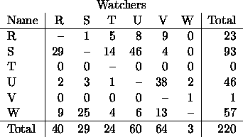
As an example, consider the following data. A colony of 6 monkeys was studied over a period of time and a record was kept of how often each monkey displayed its genitals toward each other monkey. The constraint is that monkeys cannot (at least in this experiment) display to themselves. The data appear below. Displayers

Notice that T is bashful and never displays---hence we really need to treat the entire 3rd row as well as the diagonal as structural zeros.
Now lets try to fit the quasi-independence model to these data.
402 > monkey <- fac.design(c(6,6),list(Watch=c("R","S","T","U","V","W"),
+ Display=c("R","S","T","U","V","W")))
402 > monkey$Resp <- scan("monkey.dat")
402 > monkey
   Watch Display Resp
 1     R       R    0
 2     S       R    1
 3     T       R    5
 4     U       R    8
 5     V       R    9
 6     W       R    0
 7     R       S   29
 8     S       S    0
 9     T       S   14
10     U       S   46
11     V       S    4
12     W       S    0
13     R       T    0
14     S       T    0
.........
Now set up the weights,
402 > wei <- rep(1,length(Resp))
402 > monkey[Display=="T",]
   Watch Display Resp
13     R       T    0
14     S       T    0
15     T       T    0
16     U       T    0
17     V       T    0
18     W       T    0
402 > monkey[Display==Watch,]
   Watch Display Resp
 1     R       R    0
 8     S       S    0
15     T       T    0
22     U       U    0
29     V       V    0
36     W       W    0

402 > wei[Display=="T"] <- 0
402 > wei[Display==Watch] <- 0
402 > wei
 1 2 3 4 5 6 7 8 9 10 11 12 13 14 15 16 17 18 19 20 21 22 23 24 25 26 27 28 29
 0 1 1 1 1 1 1 0 1  1  1  1  0  0  0  0  0  0  1  1  1  0  1  1  1  1  1  1  0
 30 31 32 33 34 35 36
  1  1  1  1  1  1  0
Now, try to fit the model
402 > mymod <- glm(Resp ~ Watch + Display, family=poisson, weight=wei)
402 > anova(mymod)
Analysis of Deviance Table

Poisson model

Response: Resp

Terms added sequentially (first to last)
        Df Deviance Resid. Df Resid. Dev
   NULL                    35   352.9142
  Watch 16  95.6390        19   257.2753
Display  4 122.1061        15   135.1691
This clearly fits very poorly, the residuals and fitted values provide some insight.
402 > data.frame(Display, Watch, Resp, fitted(mymod), residuals(mymod))
   Display Watch Resp fitted.mymod. residuals.mymod.
 1       R     R    0    4.61117003       0.00000000
 2       R     S    1    5.25950848      -2.28011881
 3       R     T    5    2.48072581       1.40368049
 4       R     U    8    8.21594826      -0.07567288
 5       R     V    9    6.64804865       0.86505430
 6       R     W    0    0.39577027      -0.88968564
 7       S     R   29   19.18599258       2.08150826
 8       S     S    0   21.88357619       0.00000000
 9       S     T   14   10.32171588       1.08537395
10       S     U   46   34.18462584       1.91855873
11       S     V    4   27.66096481      -5.64376708
12       S     W    0    1.64670687      -1.81477650
13       T     R    0  394.66861611       0.00000000
14       T     S    0  450.15970329       0.00000000
15       T     T    0  212.32455423       0.00000000
16       T     U    0  703.20046854       0.00000000
17       T     V    0  569.00442629       0.00000000
18       T     W    0   33.87385456       0.00000000
19       U     R    2   10.93639583      -3.32821201
20       U     S    3   12.47407192      -3.22457813
21       U     T    1    5.88358252      -2.49456075
22       U     U    0   19.48591390       0.00000000
23       U     V   38   15.76729789       4.73158037
24       U     W    2    0.93865554       0.95032975
25       V     R    0    0.22001588      -0.66334890
26       V     S    0    0.25095050      -0.70844971
27       V     T    0    0.11836455      -0.48654816
28       V     U    0    0.39201311      -0.88545256
29       V     V    0    0.31720286       0.00000000
30       V     W    1    0.01888366       2.44472583
31       W     R    9    9.65764532      -0.21409227
32       W     S   25   11.01552689       3.60687599
33       W     T    4    5.19563795      -0.54687791
34       W     U    6   17.20750128      -3.12601524
35       W     V   13   13.92368867      -0.25035727
36       W     W    0    0.82890217       0.00000000
It appears that the Display is directed toward specific members (not randomly).