Customers Who Bought This Item Also Bought
Page of
Start over
Back
-
```
##
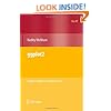
Here's the first of the also-bought books:
```
-
ggplot2: Elegant Graphics for Data …
 › ``` We _could_ extract the ISBN from this, and then go on to the next book, and so forth... ## ```0387981403,0596809158,1593273843,1449316956, 0387938362,144931208X,0387790535,0387886974,0470973927,0387759689, 1439810184,1461413648,1461471370,1782162143,1441998896,1429224622, 1612903436,1441996494,1461468485,1617291560,1439831769,0321888030,1449319793, 1119962846,0521762936,1446200469,1449358659,1935182390,0123814855,1599941651, 0387759352,1461476178,0387773169,0387922970,0073523321,141297514X,1439840954, 1612900275,1449339735,052168689X,0387781706,1584884509,0387848576,1420068725, 1441915753,1466572841,1107422221,111844714X,0716762196,0133412938,1482203537, 0963488406,1466586966,0470463635,1493909827,1420079336,0321898656,1461422981, 158488424X,1441926127,1466570229,1590475348,1430266406,0071794565,0071623663, 111866146X,1441977864,1782160604,1449340377,1449309038,0963488414,0137444265, 1461406846,0073014664,1449370780,144197864X,3642201911,0534243126,1461443423, 158488651X,1449357105,1118208781,1420099604,1107057132,1449355730,1118356853, 1449361323,0470890819,0387245448,0521518148,0521169828,1584888490,1461464455, 0387781889,0387759581,0387717617,0123748569,188652923X,0155061399,0201076160``` ## In this case there's a big block which gives us the ISBNs of _all_ the also-bought books Strategy: - Load the page as text - Search for the regexp which begins this block, contains at least one ISBN, and then ends - Extract the sequence of ISBNs as a string, split on comma - Record in a dataframe that _Data Manipulation_'s ISBN is also bought with each of those ISBNs - _Snowball sampling_: Go to the webpage of each of those books and repeat + Stop when we get tired... + Or when Amazon gets annoyed with us ## More considerations on web-scraping - You should really look at the site's `robots.txt` file and respect it - See [https://github.com/hadley/rvest] for a prototype of a package to automate a lot of the work of scraping webpages ## Summary - Loading and saving R objects is very easy - Reading and writing dataframes is pretty easy - Extracting data from unstructured sources is about using regexps appropriately + Maybe not _easy_, but at least _feasible_