% This figure plots the binomial density for four different values
% of N.  

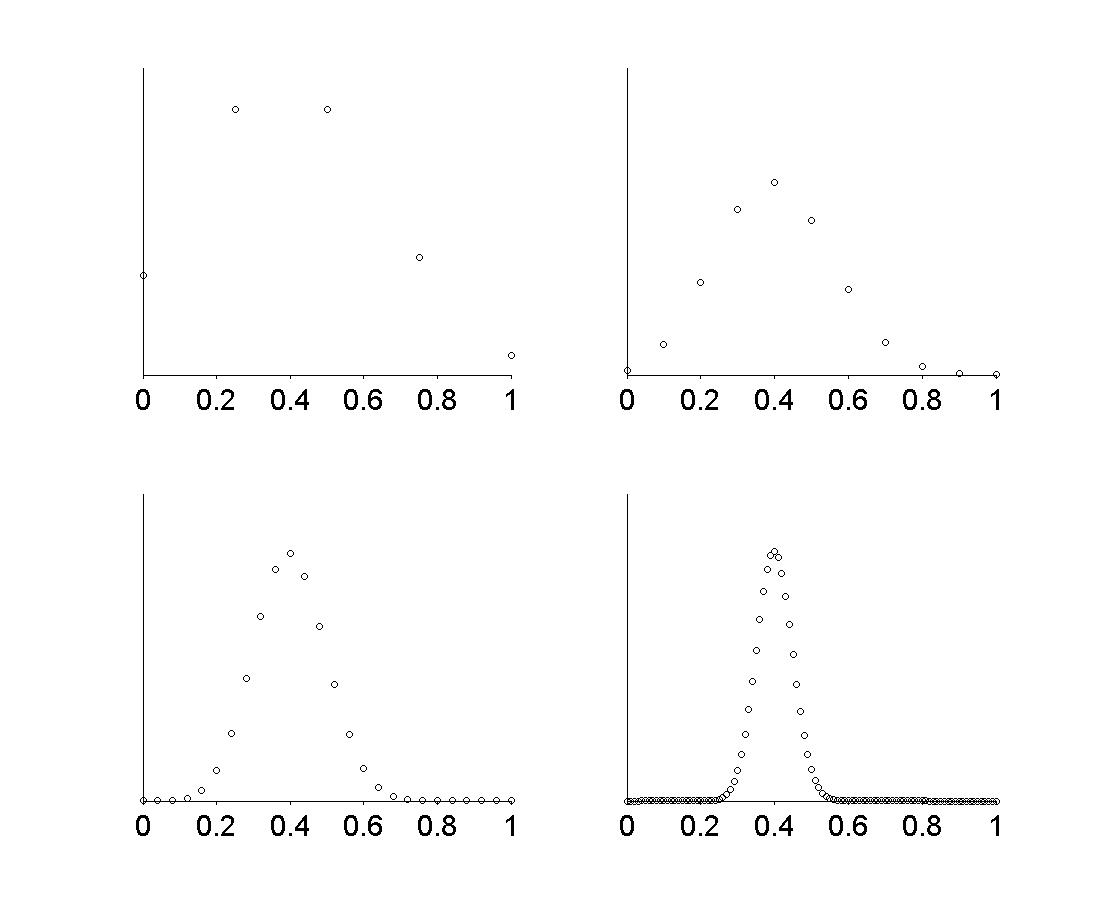
%  Figure caption: The pdf of the binomial mean X-bar when p = 0.4
%  for four different values of n.  As n increases, the
%  distribution becomes concentrated (the standard deviation of the
%  sample mean becomes small), with the center of the distribution
%  getting close to muX = 0.4 (the LLN).  In addition, the
%  distribution becomes approximately normal (the CLT).  

%  Set binomial parameters.
p = 0.4;
listOfNs = [4, 10, 25, 100];

for i = 1:4

    n = listOfNs(i);

    xValues = 0:n;
    pdfValues = binopdf(xValues, n, p);

    subplot(2, 2, i)
    plot(xValues / n, pdfValues, 'ok', 'MarkerSize', 4)
    set(gca, 'Box', 'off', 'FontSize', 18, ...
             'XTick', 0:0.2:1, 'YTick', [], 'TickDir', 'out')

end

%  Close and set figure postion. 
set(gcf, 'Position', [200, 100, 1100, 900])