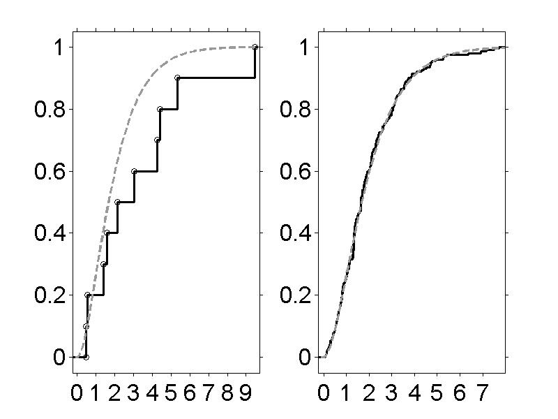
% This figure shows empirical CDFs for a small and a large sample
% from the gamma distribution to demonstrate their convergence to
% the empirical CDF.
%
%  Figure caption:  Convergence of the empirical cdf to the
%  theoretical cdf.  The left panel displays the empirical cdf for
%  a random sample of size 10 from the gamma distribution whose pdf
%  is the top right band panel of figure 3.3, together with the
%  gamma cdf.  The right panel shows the empirical cdf for a random
%  sample of size 200, again with the gamma cdf.  In the right
%  panel, the empirical cdf is quite close to the theoretical gamma
%  cdf.  

smallSample = gamrnd(2, 1, 10, 1);
largeSample = gamrnd(2, 1, 200, 1);

%  ecdf returns the empirical cdf and the values at which it's
%  evaluated.
[smallEmpiricalCDF, smallSampleXvalues] = ecdf(smallSample);
[largeEmpiricalCDF, largeSampleXValues] = ecdf(largeSample);
xValues = -.25:0.1:10;
theoreticalCDF = gamcdf(xValues, 2, 1);

figure
set(gcf, 'Position', [200, 100, 800, 600])

%%  Plot the smaller sample's empirical CDF.  %%
subplot(1, 2, 1)

%  stairs does most of our plotting, but we need to also draw lines
%  from 0 to the smallest sample, and from the largest sample out.  
stairs(smallSampleXvalues, smallEmpiricalCDF, 'k', 'LineWidth', 2)
line([-0.25, min(smallSample)], [0, 0], 'Color', 'k', 'LineWidth', 2)
line([max(smallSample), 10], [1, 1], 'Color', 'k', 'LineWidth', 2)

%  Set style parameters. 
set(gca, 'FontSize', 20, 'TickDir', 'out', ...
         'XTick', 0:1:10, 'XLim', [-0.25, max(smallSample)+0.25], ...
         'YTick', 0:0.2:1, 'YLim', [-0.05, 1.05])


hold on;
% Add circles for the actual observations.
plot(smallSampleXvalues, smallEmpiricalCDF, 'ok', 'MarkerSize', 5)

%  Add the theoretical CDF. 
plot(xValues, theoreticalCDF, '--', 'LineWidth', 2, ...
     'Color', [0.6, 0.6, 0.6])
hold off;






%%  Plot the larger sample's empirical CDF.  %%

subplot(1, 2, 2)
stairs(largeSampleXValues, largeEmpiricalCDF, 'k', 'LineWidth', 2)
line([-0.25, min(largeSample)], [0, 0], 'Color', 'k', 'LineWidth', 2)
line([max(largeSample), 10], [1, 1], 'Color', 'k', 'LineWidth', 2)

set(gca, 'FontSize', 20, 'TickDir', 'out', ...
         'XTick', 0:1:10, 'XLim', [-0.25, max(largeSample)+0.25], ...
         'YTick', 0:0.2:1, 'YLim', [-0.05, 1.05])

hold on;
%  Add the theoretical CDF.  We don't add circles at the points for
%  the large sample, since it would just clutter the figure.
plot(xValues, theoreticalCDF, '--', 'LineWidth', 2, ...
     'Color', [0.6, 0.6, 0.6])
hold off;