%  This code creates four histograms showing saccadic reaction time
%  data.  The data is the same in each histogram, but histograms 1-3
%  have different bin sizes, while histogram 4 has the same bin size
%  as histogram 3, but uses shifted bins.
%
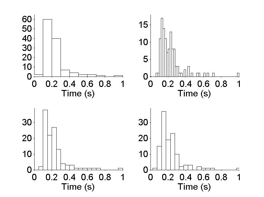
%  Figure caption: Four histograms of saccadic reaction time data.
%  The same data are used in each histogram.  The appearance of the
%  data distribution depends on details of histogram creation.  The
%  first three histograms have different bin sizes.  The fourth
%  histogram uses the same bin size as the third, but shifts the
%  bin locations slightly.  




patient1 = csvread('p3359b.csv', 0, 0);

%  Initialize a figure with four subplots.  Changing 'Position' sets
%  the position and size of the figure.  In this case, 200 pixels from
%  the left, 100 from the top, 800 pixels in width and 600 in height.
figure
set(gcf, 'Position', [200, 100, 800, 600])


%  First we set up the histogram bin locations for all four histograms.
bins = { 0.05  : 0.1  : 0.95 , ...
         0.01  : 0.02 : 0.99,  ...
         0.025 : 0.05 : 0.975, ...
         0.0   : 0.05 : 1.0  };

%  We'll also need different y limits and y tickmarks for each
%  histogram.
yLimits = { [0, 65] , [0, 18], [0, 39], [0, 39] };
yTickMarks = { 0:10:60, 0:5:15, 0:10:30, 0:10:30 };


%  We loop here so we can choose graphical parameters once, and not
%  set them repeatedly for each histogram.  
for i = 1:4

    subplot(2, 2, i)
    
    histBins   = bins{i}
    yLimits    = yLimits{i}
    yTickMarks = yTickMarcks{i}

    hist(patient1, histBins))

    %  Set graphical parameters, including the (varying) limits and
    %  tick-marks for the y-axes.  
    set(gca, 'Box', 'off', 'FontSize', 18, ...
             'XLim', [0, 1], 'Ylim', yLimits, ...
             'XTick', 0:0.2:1, 'YTick', yTickMarks, 'TickDir', 'out')
    
    %   The next two lines find the handle of the plotted object (called a
    %   "patch") and set its color to white ('w').  These are the same in each
    %   histogram.
    spikehist = findobj(gca, 'Type', 'patch');
    set(spikehist, 'FaceColor', 'w')
    xlabel({'Time (s)'}, 'FontSize', 18)
    

end