%%  Simulates Galton father/son data (see Friedman 78).

%% First set some graphical parameters
scatterPointSize = 6;
conditionalMeanMarkerSize = 10;


%  Set bivariate normal parameters (from Freedman)
N   = 100;
xMu = 68; yMu = 69;
xSD = 2.7; ySD = 2.7;
rho = 0.5;
covariance = rho * xSD * ySD;

%  Set up arrays for function inputs. 
mu = [xMu, yMu]; sigma = [xSD^2, covariance; covariance, ySD^2];

%  Draw a random sample
Nsample = 1078;
sample = mvnrnd(mu, sigma, Nsample);

%  Fit a linear model.  
lmgalton = polyfit(sample(:, 1), sample(:, 2), 1);



%%%%%%%%%%%%%%%%%%%%%%%%%%%%%%%%%%%%%%%%%%%%%%%%%%%%%%%%%%%%%%%%%%%%%%%%%%%%%%%%
%%%%%%%%%%%%%%%%%%%% First create the level sets plot %%%%%%%%%%%%%%%%%%%%%%%%%%
%%%%%%%%%%%%%%%%%%%%%%%%%%%%%%%%%%%%%%%%%%%%%%%%%%%%%%%%%%%%%%%%%%%%%%%%%%%%%%%%

%  Set levels for the level set plot.  
levels = [0.8, 0.9, 0.95, 0.99];
inverseSigma = sigma^-1;
cband_y = sqrt(chi2inv(levels, 2)/inverseSigma(1,1));

confidenceBandPoints = [68+cband_y; 69+zeros(1, 4)]';
confidenceBandValues = mvnpdf(confidenceBandPoints, mu, sigma);

xgrid = (xMu-(3.5*xSD)):(7*xSD/N):(xMu+(3.5*xSD));
ygrid = (yMu-(3.5*ySD)):(7*ySD/N):(yMu+(3.5*ySD));

[x, y] = meshgrid(xgrid, ygrid);
pdfValues = mvnpdf([x(:), y(:)], mu, sigma);
pdfValues = reshape(pdfValues, size(x));

figure
set(gcf, 'Position', [200, 200, 1700, 600])
subplot(1, 2, 1)

[C,h] = contour(xgrid, ygrid, pdfValues, ...
                'LevelList', confidenceBandValues, 'LineWidth', 2);

%  Add in text labels for level sets.

v = {'80%', '90%', '95%', '99%'};
textHandles = clabel(C, h, 'FontSize', 15, 'LabelSpacing', 2000);
m = length(textHandles);
for i = 1:m
  set(textHandles(i), 'String', v(i));
end



set(h,'ShowText','off')
colormap gray(1)
set(gca, 'FontSize', 20, 'xlim', [58, 78], 'ylim', [59, 79], 'TickDir', 'out')
xlabel('Father''s Height (inches)', 'FontSize', 20)
ylabel('Son''s Height (inches)', 'FontSize', 20)




%%%%%%%%%%%%%%%%%%%%%%%%%%%%%%%%%%%%%%%%%%%%%%%%%%%%%%%%%%%%%%%%%%%%%%%%%%%%%%%%
%%%%%%%%%%%%%%%%%%%% Create the scatter plot %%%%%%%%%%%%%%%%%%%%%%%%%%%%%%%%%%%
%%%%%%%%%%%%%%%%%%%%%%%%%%%%%%%%%%%%%%%%%%%%%%%%%%%%%%%%%%%%%%%%%%%%%%%%%%%%%%%%




subplot(1, 2, 2)

plot(X(:, 1), X(:, 2), '.', ... 
     'MarkerSize', scatterPointSize, 'MarkerEdgeColor', [0.6, 0.6, 0.6])
set(gca, 'FontSize', 20, 'xlim', [58, 78], 'ylim', [59, 79], 'TickDir', 'out')
xlabel('Father''s Height (inches)', 'FontSize', 20)
ylabel('Son''s Height (inches)', 'FontSize', 20)





%%%%%%%%%%%%%%%%%%%%%%%%%%%%%%%%%%%%%%%%%%%%%%%%%%%%%%%%%%%%%%%%%%%%%%%%%%%%%%%%
%%%%%%%%%%%%%%%%%%%% Add lines to both %%%%%%%%%%%%%%%%%%%%%%%%%%%%%%%%%%%%%%%%%
%%%%%%%%%%%%%%%%%%%%%%%%%%%%%%%%%%%%%%%%%%%%%%%%%%%%%%%%%%%%%%%%%%%%%%%%%%%%%%%%


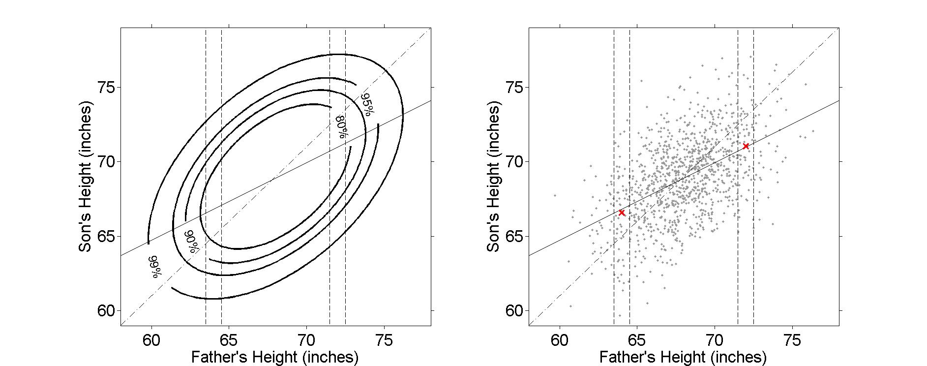
%  In the next section, we choose two points, at father's heights
%  of 64 and 72 inches, and plot the mean of the observations
%  falling within a small window of those points.  The goal is to
%  show that the conditional means are close to the regression
%  line.  

%  Set the points
point1x = 64;
point2x = 72;

%  Create small windows.
epsilon = 0.5;
window1 = point1x + epsilon * [-1, 1];
window2 = point2x + epsilon * [-1, 1];

%  Find Xs close to the point's xs.
inWindow1 = abs( sample(:,1) - point1x ) < epsilon;
inWindow2 = abs( sample(:,1) - point2x ) < epsilon;

%  Find the mean Ys for Xs close to point's xs.  
point1y = mean( sample( inWindow1, 2 ) );
point2y = mean( sample( inWindow2, 2 ) );

%  Now go through and add the lines and points. 
for i = 1:2

    subplot(1,2,i)
    set(gca,'OuterPosition',get(gca,'OuterPosition')+[0, 0+0.05, 0, 0])
    hold on;
    %  Draw the vertical lines creating boundaries around the small
    %  windows.
    %  line([x1, x2], [y1, y2]) plots a line from x1,y1 to x2,y2, so
    %  line([x, x], [yLow, yHigh]) plots a vertical line at x.
    lineLocations = [window1, window2];
    yLimits = [50, 90];
    for j = 1:4
        line([lineLocations(j), lineLocations(j)], yLimits, ...
             'Color', 'k', 'LineStyle', '--')
    end
    
    
    %  The theoretical line has slope 1 and intercept 1 (means are 69
    %  and 68, so sons are, on average, 1 inch taller than fathers).
    theoreticalLine = refline(1, 1);
    regressionLine = refline(lmgalton(1, 1), lmgalton(1, 2));
    set(theoreticalLine, 'Color', [0, 0, 0], 'LineStyle', '-.')
    set(regressionLine, 'Color', [0, 0, 0])
    
    %  Place xs ('xr' symbols) at the conditional means.  
    plot([point1x, point2x], [point1y, point2y], 'xr', ...
         'LineWidth', 2, 'MarkerSize', conditionalMeanMarkerSize)
    
end