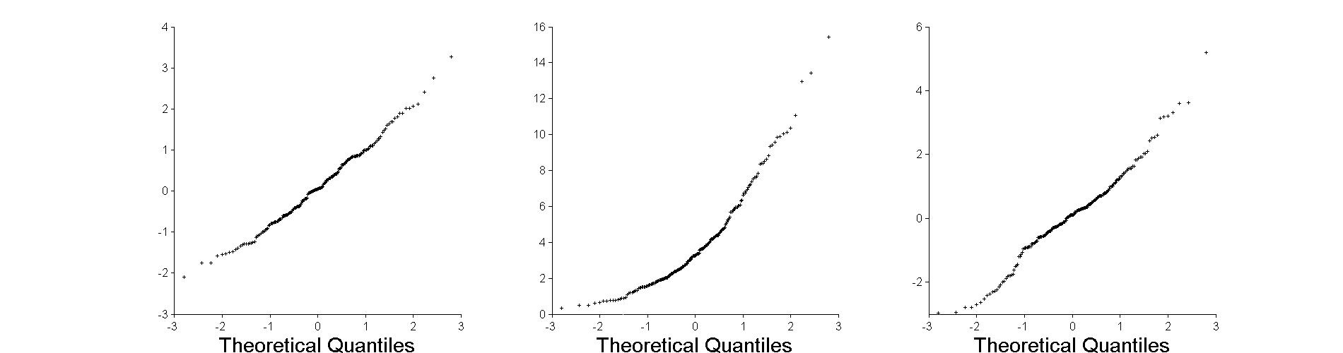
%  This script plots three QQ-normal plots, for a normal, gamma,
%  and t distribution.   

%  Set up the figure.
figure
set(gcf, 'Position', [0, 200, 1900 500])
fontSize = 18;  
markerSize = 3;

%  Set simulation parameters.
N = 200
%  ProbDistUnivParam is a Matlab function to create a probability
%  distribution object.  It's used in the qq plotting function.
standardNormal = ProbDistUnivParam('normal', [0, 1]);

%  Draw the samples for the empircal CDFs.  
normalSample = normrnd(0, 1, N, 1);
chiSquaredSample = chi2rnd(4, N, 1);
tSample = trnd(3, N, 1);

%  Plot the QQ normal for a normal sample.  
subplot(1, 3, 1)
qqNormal = qqplot(normalSample, standardNormal);
set(qqNormal, 'Color', 'w', 'MarkerSize', markerSize, 'MarkerEdgeColor', 'k')
set(gca, 'XTick', -4:1:4, 'YTick', -4:1:4, 'TickDir', 'out')
xlabel('Theoretical Quantiles', 'FontSize', fontSize)
ylabel('')
title('')

%  Plot the QQ normal for a chi squared sample. 
subplot(1, 3, 2)
qqChiSquared = qqplot(chiSquaredSample, standardNormal);
set(qqChiSquared, 'Color', 'w', 'MarkerSize', markerSize, 'MarkerEdgeColor', 'k')
set(gca, 'XTick', -4:1:4, 'YTick', 0:2:18, 'TickDir', 'out')
ylim([0, ceil(max(chiSquaredSample))])
xlabel('Theoretical Quantiles', 'FontSize', fontSize)
ylabel('')
title('')

%  Plot the QQ normal for a t sample.  
subplot(1, 3, 3)
qqT = qqplot(tSample, standardNormal);
set(qqT, 'Color', 'w', 'MarkerSize', markerSize, 'MarkerEdgeColor', 'k')
set(gca, 'XTick', -4:1:4, 'YTick', -8:2:8, 'TickDir', 'out')
xlabel('Theoretical Quantiles', 'FontSize', fontSize)
ylabel('')
title('')