#   Code by Rob Kass, revised by Patrick Foley
#
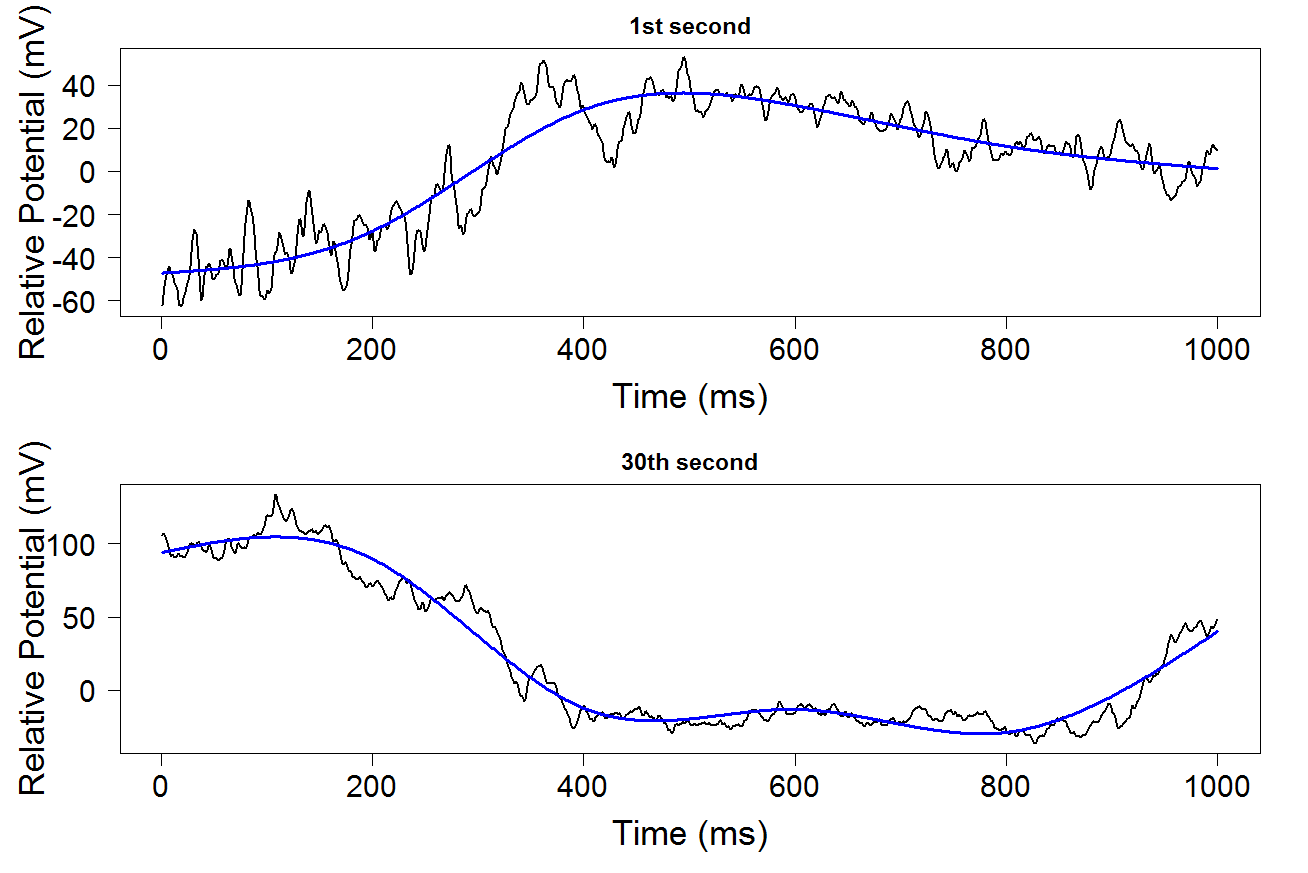
#   Data from Ryan Kelly --- average of
#   96 LFPs taken from Utah array in V1
#   of anesthetized monkey while shown
#   blank screen (baseline condition).
#   Data are sampled at 1KHz for 30 seconds.


#  Figure 18.1 shows the spline-averaged trend of the first and
#  thirtieth seconds of data.  We first read in the data and set up a
#  jpeg.
lfp <- read.table("data/lfp-ryan.dat")[,1]
jpeg("figure18.1.jpeg")

time <- 1:1000
lfp.1stSecond <- lfp[1:1000]
lfp.30thSecond <- lfp[29001:30000]


#  Fit a spline model with four knots, evenly spaced.
library("splines")
knotTimes <- c(200, 400, 600, 800)
splineModel1 <- lm(lfp.1stSecond ~ ns(time, knots = knotTimes))
splineModel30 <- lm(lfp.30thSecond ~ ns(time, knots = knotTimes))

#  Pull the fits, giving fit values for LFP at each time.
splineFit1 <- splineModel1$fit
splineFit30 <- splineModel30$fit

#  Set graphical parameters (the size of "labal" and "axis", and then
#  the style of the axis).
par(cex.lab = 1.75)
par(cex.axis = 1.5)
par(las = 1)

#  Now set the graphical parameter to allow for two rows of graphs.
par(mfrow = c(2,1))
par(mar = c(5, 5, 2, 2))

#  For the first second, plot the data and then add lines at the spline fits.
plot(time, 
	lfp.1stSecond, 
	type = "l", 
	lwd = 2, 
	xlab = "Time (ms)", 
	ylab = "Relative Potential (mV)",
	main = "1st second")
lines(time, splineFit1, col = "blue", lwd = 3)

#	And do the same for the 30th second.
par(cex.lab=1.75)
par(cex.axis=1.5)
par(las=1)
plot(time, 
	lfp.30thSecond, 
	type = "l", 
	lwd = 2, 
	xlab = "Time (ms)", 
	ylab = "Relative Potential (mV)",
	main = "30th second")
lines(time, splineFit30, col = "blue", lwd = 3)

#	With the jpeg finished, we close the graphical device.
dev.off()