# Code initially written by Rob Kass, revised by Patrick Foley.

#  First read in the temperature data, and assign column names.
temperatureDF <- read.table("data/temp.dat",col.names=c("Temp","Time"))
temperature <- temp$Temp
time <- temp$Time

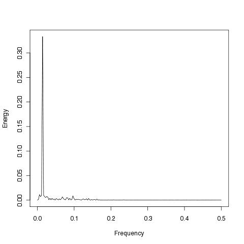
#  Now we make the Periodogram, found in figure 18.4.
#  Our periodogram looks slightly different from that in the book.
#  The book rescales energies.
n <- length(temperature)

#  Now we recenter temperature around 0 (otherwise the periodogram
#  would have a (possibly large) component at 0 which could dwarf the
#  interesting spectral behavior).
centeredtemperature <- temperature - mean(temperature)

#  We find the total energy, take the fourier transform, and scale to
#  appropriate energy.
totalVariance <- sum(centeredtemperature^2)
temperatureDFT <- fft(centeredtemperature)
dftEnergies <- abs(temperatureDFT)^2
R2s <- dftEnergies / sum(dftEnergies)


jpeg("figure18.4.jpg")
frequencies <- 0:(n/2) / n
plot(frequencies,
     R2s[1:((n/2)+1)],
     type = "l",
     xlab = "Frequency",
     ylab = "Energy")
dev.off()