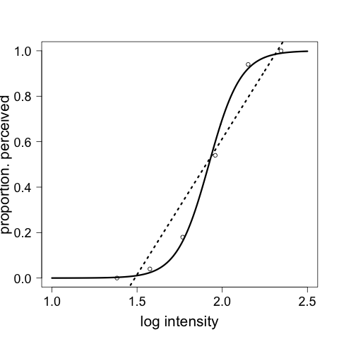
#  Figure caption: proportionortion of trials, out of 50, on which
#  light flashes were perceived by subject S.S. as a function of log10
#  intensity, together with fits.  Data from Hecht et al (first seris
#  of trials) are shown as circles.  Dashed line is the fit obtained
#  by linear regression.  Solid curve is the fit obtained by logistic
#  regression.

expit <- function(x) { exp(x) / (1 + exp(x)) }

responses <- c(0, 2, 9, 27, 47, 50)
noresponses <- 50 - responses
proportion <- responses / 50

percept <- cbind(responses, noresponses)
intensity<- log(c(24.1, 37.6, 58.6, 91, 141.9, 221.3), 
                base = 10)

subject1.df <- data.frame(intensity,percept)
subject1.lm <- lm(proportion ~ intensity)
subject1.glm <- glm(percept ~ intensity,
                    family = binomial,
                    data = subject1.df)

x <- seq(1, 2.5, by = .01)
linearRegressionLine <- 
  subject1.lm$coef[1] + subject1.lm$coef[2]*x
logisticRegressionLine <- 
  expit(subject1.glm$coef[1]+subject1.glm$coef[2]*x)

png("../figures/hechtSS.png")
par(cex.lab=1.75)
par(cex.axis=1.5)
par(las=1)
plot(intensity, proportion,
    xlim = c(1, 2.5), ylim = c(0, 1), 
     xlab = "log intensity", ylab = "proportion. perceived")

lines(x, linearRegressionLine, lwd=3, lty=3)
lines(x, logisticRegressionLine, lwd=3)

dev.off()

#  The analysis below is not necessary for creating the figure.
summary(subject1.lm)
summary(subject1.glm)
b0<-subject1.glm$coef[1]
b1<-subject1.glm$coef[2]

vmatr<-summary(subject1.glm)$cov.unscaled
dg1<- -1/b1
dg2<- b0/b1^2
x50<- -b0/b1
se<-sqrt(crossprod(c(dg1,dg2), vmatr %*% c(dg1, dg2)))
library(MASS) # needed for mvrnorm
beta<- mvrnorm(10000, c(b0,b1), vmatr)
x50vec<- -beta[,1] / beta[,2]
sqrt(var(x50vec))