#  Code initially written by Ryan Sieberg.

#  First set up a PNG graphics device in which we will print the image.
png("../figures/hurshR.png")

#  Read data from CSV.
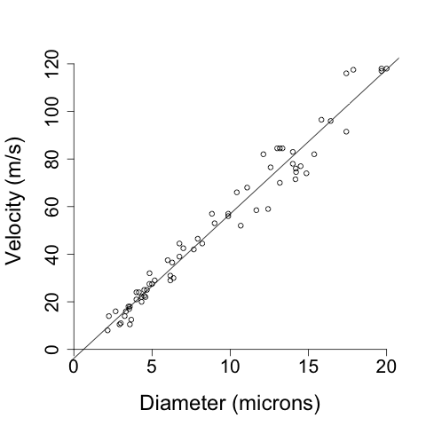
hursh <- read.csv("../data/hursh.csv")
#  hursh contains two named columns, 'diameter' and 'velocity'.

#  The 'par' commands change graphical parameters.  cex stands for
#  "character expansion" and determines the size of text, in this
#  case, cex.lab changes the size of the label.
par(cex.lab=2)
#  cex.axis changes the size of the axis font.
par(cex.axis=1.75)
#  mar changes the margins of the graph area.
par(mar=(c(5,4.7,4,2)+.1))

#  Create a linear model for the hursh data.
lmhursh<-lm(hursh$velocity ~ hursh$diameter)

# Plot the data.
plot(hursh$diameter,
     hursh$velocity,
     main="",
     axes=FALSE,
     xlab="Diameter (microns)",
     ylab="  Velocity (m/s)",
     xlim=c(0,20),
     ylim=c(0,120))

axis(1,pos=0)
axis(2,pos=0)

#  Add a line.  The linear model object "lmhursh" contains a list
#  called "coef", which contains the coefficients of the model.  The
#  first entry is the intercept, and the second is the coefficient for
#  velocity.  They are stored as strings, so we convert them to
#  numerics before using them in abline.
intercept <- as.numeric(lmhursh$coef[1])
slope <- as.numeric(lmhursh$coef[2])
abline(intercept, slope, untf = "FALSE")

#  With our figue complete, close the connection to the PNG.
dev.off()