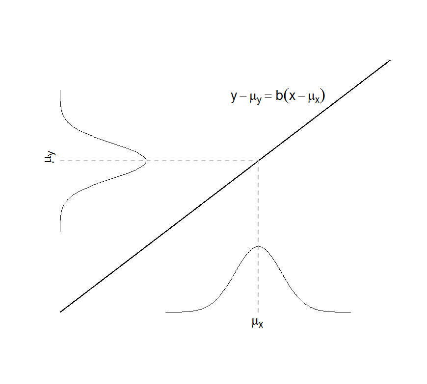
#
#
#  Figure caption:  The effect of the transformation y = a + bx
#  operating on a normally distributed random variable X having
#  mean muX and standard deviation sigmaX.  The random variable Y =
#  a + bX is again normally distributed, with mean muY = a + b*muX
#  and standard deviation sigmaY = |b| sigmaX.  The normal
#  distributions are displayed on the x and y axes; the linear
#  transformation is displayed as a line, which passes through the
#  point (muX, muY) so that it may be written, equivalently, as y -
#  muY = b(x - muX).
#
#  For Y = a + b*X,  we use a = 0, b = 0.7.  
a <- 0
b <- 0.7

#  Set up the normal random variable X. 
x.mu <- 3
x.sd <- 0.35

#  Set up Y as the transformation of X. 
y.mu <- b * x.mu + a
y.sd <- abs(b) * x.sd

x.max <- 2 * x.mu                   #  Used for setting x-axes.

#  Get a reasonable range of values and evaluate the PDFs.
x.values <- seq(from = x.mu - 4 * x.sd, to = x.mu + 4 * x.sd, by = 0.01)
y.values <- a + b * x.values

par(xaxs = "i")
par(yaxs = "i")
par(oma = rep(1, 4))

#  Open an empty plot and set some axes.
plot(0, 0, type = "n", xlim = c(0, 5), ylim = c(0, 3.5),
     xaxt = "n", xlab = "", yaxt = "n", ylab = "",
     main = "", bty = "n")

#  Add lines for X and Y's PDFs.  
lines(x.values, dnorm(x.values, x.mu, x.sd) * 0.8, lwd = 1.5)
lines(dnorm(y.values, y.mu, y.sd) * 0.8, y.values, lwd = 1.5)

#  Add a line showing the relationship between X and Y.  
lines(c(0, 5), c(0, a+b*5), lwd = 2)
#  Add lines from the means of X and Y to the line showing their relationship.
lines(c(x.mu, x.mu), c(0, y.mu), col = "gray", lty = 2, lwd = 2)
lines(c(0, x.mu), c(y.mu, y.mu), col = "gray", lty = 2, lwd = 2)

#  Set labels.
text(3.3, 3, expression(y-mu[y] == b(x-mu[x])), cex = 1.4)
#  (expression(phanton(  ) ) is empty space)
title(xlab = expression(paste(phantom(xxxxxxxxxx), mu[x])), line=0.5, cex.lab=1.4)
title(ylab = expression(paste(phantom(xxxxxxxxx), mu[y])), line=0.2, cex.lab=1.4)

#  Close the graphics device
png("figure9.1.png")