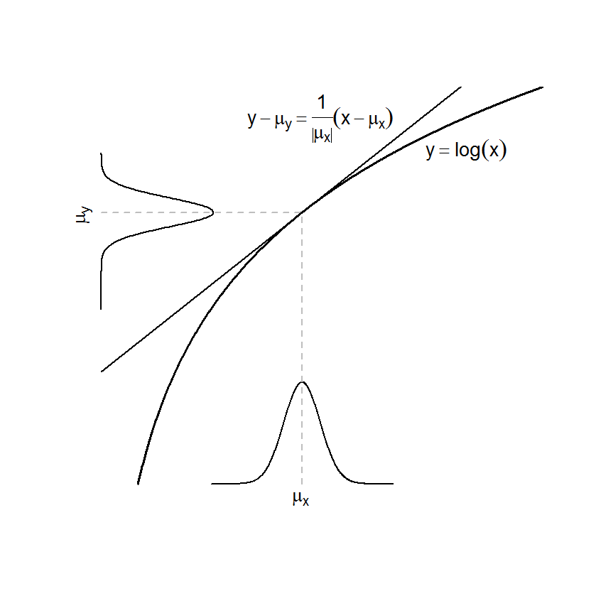
#  This plot shows the effect of a linear transform to a normal 
#  random variable.

sd.neighborhood <- 5       #  We'll polot +/- this many SDs
x.mu <- 5.5
x.sd <- 0.5
y.mu <- log(x.mu)
y.sd <- x.sd / abs(x.mu)
x.values<-seq(from = x.mu - sd.neighborhood * x.sd, 
           to = x.mu + sd.neighborhood * x.sd, by = 0.01)
y.values <- log(x.values)

x.max <- 2.2 * x.mu

#  Set graphical parameters.  
par(xaxs = "i")
par(yaxs = "i")
par(oma = rep(1, 4))
line.width <- 2

#  Set up the plot.
plot(0, 0, type = "n", 
     xlim = c(-0.4, x.max), ylim = c(-0.05, log(x.max)), 
     xaxt = "n", xlab = "", yaxt = "n", ylab = "", main = "", bty = "n")
#  Add the horizontal density, x, and then the vertical density, y, which is
#  a linear transformation of x.  
lines(x.values, 0.8*dnorm(x.values, x.mu, x.sd), lwd = line.width)
lines(0.7*dnorm(y.values, y.mu, y.sd), y.values, lwd = line.width)

#  Add lines 
logvals<-seq(1, x.max, by = 0.01)
lines(logvals, log(logvals), lwd = 3)
lines(c(0, x.max), 
      c(y.mu - sign(x.mu), (x.max/abs(x.mu)) + y.mu - sign(x.mu)),
      lwd = line.width)
lines(c(x.mu, x.mu), c(0, y.mu), col = "gray", 
      lty = 2, lwd = line.width)
lines(c(0, x.mu), c(y.mu, y.mu), col = "gray", 
      lty = 2, lwd = line.width)

text(6, 2.3, expression(y-mu[y] == frac(1, abs(mu[x]))(x-mu[x])), cex = 1.4)
text(10, 2.1, expression(y == log(x)), cex = 1.4)


title(xlab = expression(paste(mu[x], phantom(xxx))), line=0, cex.lab=1.4)
title(ylab = expression(paste(phantom(xxxxxxxxxxxxxxxx), mu[y])), line=-0.5, cex.lab=1.4)

#  Close the graphics device
png("figure9.2.png")