#  Creates a figure showing a binomial pdf overlapping the normal
#  approximation to a binomial.
#
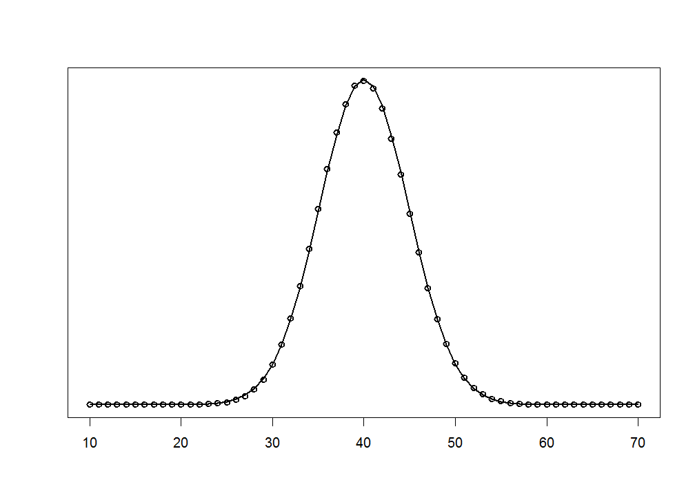
#  Figure caption:  The normal approximation to the binomial.
#  Black circles are pdf values for a B(100, 0.4) distribution;
#  the solid line is the pdf of a normal having the same mean and variance.

postscript("normbinom.ps")

xvals <- c(10:70)

# Set binomial parameters.
n <- 100
p <- 0.4
binomialMean <- n * p
binomiealVariance <- n * p * (1 - p)

# Plot points at the binomial pdf values.  
plot(xvals, dbinom(xvals, p = p, size = n),
     xlab = "", ylab = "", lwd = 2, yaxt = "n")

# Plot a line through the normal pdf. 
lines(xvals, dnorm(xvals, mean = binomialMean, sd = sqrt(binomialVariance)),
      lwd=2)

dev.off()