Initial Analysis and ANOVA table: cell means model

The following data is from Box, Hunter and Hunter (1978) and is also analyzed in Chapter 13 of the SPLUS Guide to Statistics. It gives blood coagulation times for each of four diets.

We enter the data more or less as in the SPLUS manual,

402 > coag.times _ scan()
1: 62 63 68 56
5: 60 67 66 62
9: 63 71 71 60
13: 59 64 67 61
17: 65 68 63
20: 66 68 64
23: 63
24: 59
25: 
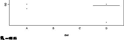
402 > diet _ factor(c(rep(LETTERS[1:4],4),rep(LETTERS[1:3],2),c("A","A")))
402 > split(coag.times,diet)  # check that the factor labels are right
$A: [1] 62 60 63 59 65 66 63 59
$B: [1] 63 67 71 64 68 68
$C: [1] 68 66 71 67 63 64
$D: [1] 56 62 60 61
402 > sapply(split(coag.times,diet),mean)
      A        B    C     D 
 62.125 66.83333 66.5 59.75
402 > coag _ data.frame(coag=coag.times,diet=diet)

Now we fit the model, look at some diagnostic plots, and consider the analysis of variance table. More details on the SPLUS parts of the problem can be found in Chapter 13 of the SPLUS Guide to Statistics.

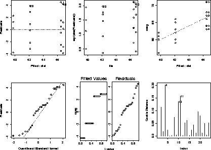
402 > coag.aov _ aov(coag ~ diet, data=coag)
402 > par(mfrow=c(2,3))
402 > plot(coag.aov)

402 > model.tables(coag.aov,type="means")
Refitting model to allow projection
Tables of means
Grand mean      

 64

 diet 
        A     B    C     D 
    62.12 66.83 66.5 59.75
rep  8.00  6.00  6.0  4.00

The cell means and the grand mean are illustrated in the figure below; the cell means are the estimates of the 's in the cell means model

where k is the number of cells, and there are observations in the cell. As usual in regression, the error terms ( in this case) are distributed for some unknown error variance .

=1in

Now recall that we can write the deviation of a single observation from the grand mean as

If we square and sum these terms, the magic of orthogonal sums of squares tells us

with degrees of freedom n-1, n-k and k-1 respectively. This gives rise to the ANOVA table

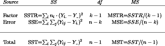
Here is SPLUS's ANOVA table for this ANOVA model.

402 > anova(coag.aov)     # some output omitted below
Terms added sequentially (first to last)
          Df Sum of Sq  Mean Sq  F Value       Pr(F) 
     diet  3  186.0417 62.01389 8.055931 0.001028171
Residuals 20  153.9583  7.69792                     
402 >  186.0417 /( 186.0417 +153.9583)  # R^2
[1] 0.5471815

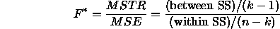
Under the null hypothesis

is distributed as . Large values of argue in favor of