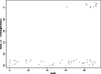
Look at the stroke data. This is explicitly 0--1 data, and it is very hard to think about plotting it. A simple plot of, say, Status against WAB1, looks like the following, and it not all that informative.
402 > plot(WAB1, Status)

Even if I jitter the points a little, it is still not very easy to see any trends or patterns.
402 > plot(WAB1, Status+0.1*runif(length(Status)))
A somewhat more useful approach is to plot the data and add some sort of smooth curve that will allow you to at least look at some of the trends in the data. The particular approach I took with these data was to superimpose a (black-box) smooth curve generated by loess. The various pictures result from different smoothing parameters.
402 > scatter.smooth(WAB1, Status,span=0.2)
402 > title("Span = 0.2")
402 > scatter.smooth(WAB1, Status,span=0.35)
402 > title("Span = 0.35")
402 > scatter.smooth(WAB1, Status,span=0.5)
402 > title("Span = 0.5")
402 > scatter.smooth(WAB1, Status,span=0.65)
402 > title("Span = 0.65")
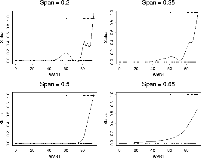
This is still not perfect, but you certainly get the sense that the probability goes up, probably more or less monotonely with WAB1.
Compare this to the similar picture(s) for Age.
402 > for (i in c(0.2, 0.35, .5, 0.65)){
+ scatter.smooth(Age, Status, span=i)
+ title(paste("Span = ", i))
+ }

If anything, there is a bit of evidence for some type of quadratic effect of Age, but the probable story is that Age is not that important, on its own. We should always remember that variables that do not seem to be important (from these marginal plots), may be quite important when paired with other variables (that is viewed conditionally).
With that hint about the Age variable, I re-ran the logistic regression model for these data and obtained,
402 > mymod <- glm(Status ~ Side + Gender + LOSD +WAB1 + Age + Age^2, family=bin>
402 > summary(mymod)

Call: glm(formula = Status ~ Side + Gender + LOSD + WAB1 + Age + Age^2, family =
        binomial)
Deviance Residuals:
       Min         1Q        Median            3Q      Max
 -1.317304 -0.2637303 -0.0002506098 -6.014239e-07 2.770847

Coefficients:
                   Value   Std. Error   t value
(Intercept) -42.13652444 17.240544854 -2.444037
       Side  -1.70612965  1.320176507 -1.292350
     Gender   4.03384776  1.847166535  2.183803
       LOSD  -0.28388626  0.130491084 -2.175522
       WAB1   0.24891576  0.104667163  2.378165
        Age   0.92453559  0.421765743  2.192059
   I(Age^2)  -0.00791642  0.003578441 -2.212254

(Dispersion Parameter for Binomial family taken to be 1 )

    Null Deviance: 65.71913 on 60 degrees of freedom

Residual Deviance: 21.7621 on 54 degrees of freedom

402 > anova(mymod)
Analysis of Deviance Table

Binomial model

Response: Status

Terms added sequentially (first to last)
         Df Deviance Resid. Df Resid. Dev
    NULL                    60   65.71913
    Side  1  0.10011        59   65.61902
  Gender  1  3.36010        58   62.25892
    LOSD  1 13.46451        57   48.79441
    WAB1  1 19.75552        56   29.03889
     Age  1  0.05110        55   28.98780
I(Age^2)  1  7.22570        54   21.76210
This is somewhat surprising (because I didn't think there was an Age effect). Could we have seen the same trend from a residual analysis of these data?
Let us go back to the original model and look at residuals.

There is at least one large (Pearson) residual, and it is the same point as the large (deviance) residual. What about a plot of (deviance) residual against Age (when Age is in the model).
402 > mymod <- glm(Status ~ Side + Gender + LOSD +WAB1 + Age, family=binomial)
402 > scatter.smooth(Age, (residuals(mymod)))
402 > identify(Age, (residuals(mymod)))
[1] 59
402 > scatter.smooth(Age[-59], (residuals(mymod))[-59])
We see that observation 59 is the one with the large residual. If I plot the data (the lower plot) without that observation, the quadratic trend seems to go away, at least a bit.

Observation 59 is now suspect, so let us remove that observation, and see what the resulting model looks like.
402 > WW <- rep(1, length(Side))
402 > WW[59] <- 0
402 > mymod <- glm(Status ~ Side + Gender + LOSD +WAB1 + Age,
+ weight=WW, family=binomial)
Warning messages:
  linear convergence not obtained in  10  iterations. in: glm.fitter(x = X, y =
        Y, w = w, start = start, offset = offset, family = family, ....
Oh-oh, what does that mean? (Basically, the optimization algorithm is converging slowly, which is an indication that there are some fitted probabilities that are very close to 0 or 1). We can try a few more iterations, via.
402 > mymod <- glm(Status ~ Side + Gender + LOSD +WAB1 + Age,
+ weight=WW, maxit=30,family=binomial)
Now, what does the summary and anova look like?
402 > summary(mymod)

Call: glm(formula = Status ~ Side + Gender + LOSD + WAB1 + Age, family = binomial,
        weights = WW, maxit = 30)
Deviance Residuals:
      Min           1Q        Median            3Q      Max
 -1.21685 -0.006138687 -2.107342e-08 -2.107342e-08 2.120409

Coefficients:
                    Value  Std. Error     t value
(Intercept) -46.034665461 23.60416082 -1.95027757
       Side  -7.479606389  4.79366143 -1.56031178
     Gender   7.889726328  4.28891089  1.83956406
       LOSD  -0.677382165  0.43418335 -1.56012928
       WAB1   0.662724777  0.34770876  1.90597667
        Age  -0.001289562  0.04096666 -0.03147832

(Dispersion Parameter for Binomial family taken to be 1 )

    Null Deviance: 62.71879 on 60 degrees of freedom

Residual Deviance: 13.32727 on 54 degrees of freedom

Number of Fisher Scoring Iterations: 10

Correlation of Coefficients:
       (Intercept)       Side     Gender       LOSD       WAB1
  Side  0.8469550
Gender -0.9187997  -0.8860396
  LOSD  0.7944690   0.9174434 -0.8555061
  WAB1 -0.9831416  -0.9061715  0.9317554 -0.8758313
   Age -0.0387868   0.0615410  0.0243350 -0.0022418 -0.0596445
Warning messages:
  1 rows with zero weights not counted in: summary(mymod)
If I now start adding the quadratic term in Age, I get myself into all sorts of trouble.
402 > formula(mymod)
Status ~ Side + Gender + LOSD + WAB1 + Age + Age^2
402 > anova(mymod)
Analysis of Deviance Table

Binomial model

Response: Status

Terms added sequentially (first to last)
         Df Deviance Resid. Df Resid. Dev
    NULL                    60   62.71879
    Side  2  0.62858        58   62.09021
  Gender  1  2.34693        57   59.74328
    LOSD  1 13.67051        56   46.07277
    WAB1  1 32.74451        55   13.32826
     Age  1  0.00099        54   13.32727
I(Age^2)  1 13.32727        53    0.00000
Warning messages:
1: linear convergence not obtained in  10  iterations. in: glm.fit(x, y, w,
        offset = offset, family = family, maxit = control$maxit,  ....
2: linear convergence not obtained in  10  iterations. in: glm.fit(x, y, w,
        offset = offset, family = family, maxit = control$maxit,  ....
Whoa. What is going on here? We suddenly have a model that fits perfectly?
The summary looks even weirder?
402 > summary(mymod)

Call: glm(formula = Status ~ Side + Gender + LOSD + WAB1 + Age + Age^2, family =
        binomial, weights = WW, maxit = 50)
Deviance Residuals:
         Min            1Q        Median            3Q          Max
 -3.9065e-05 -2.107342e-08 -2.107342e-08 -2.107342e-08 3.281089e-05

Coefficients:
                    Value  Std. Error       t value
(Intercept) -2858.6085408 2227320.001 -0.0012834297
       Side  -164.0618144  165491.082 -0.0009913635
     Gender   273.5752941  237195.052  0.0011533769
       LOSD   -16.2464405   13633.473 -0.0011916582
       WAB1    24.1122280   17153.825  0.0014056473
        Age    39.8782980   35880.527  0.0011114190
   I(Age^2)    -0.3549147     302.566 -0.0011730157

(Dispersion Parameter for Binomial family taken to be 1 )

    Null Deviance: 62.71879 on 60 degrees of freedom

Residual Deviance: 0 on 53 degrees of freedom

Number of Fisher Scoring Iterations: 29

Correlation of Coefficients:
         (Intercept)       Side     Gender       LOSD       WAB1        Age
    Side  0.3661039
  Gender -0.8397332  -0.5132934
    LOSD  0.7676113   0.5867586 -0.7405370
    WAB1 -0.9678428  -0.5023038  0.8384746 -0.7822973
     Age -0.9537356  -0.2802197  0.7986261 -0.8085521  0.8643352
I(Age^2)  0.9585630   0.3372172 -0.8129406  0.8428222 -0.8863173 -0.9963403
Warning messages:
1: fitted values close to 0 or 1 in: family$deviance(mu, y, w, residuals = T)
2: 1 rows with zero weights not counted in: summary(mymod)
402 >
On reflection, it is clear what is going on. Look at the first plot of Status against WAB1. Here we see, that absent the one observation in the middle (which is 59), we have an almost perfect discimination between the two levels of Status. That is the clue to what is ``broken''. With the 7 parameters (anything like WAB1 squared would have done), we can find a function that perfectly discriminates between the two levels of status, and then maximum likelihood modelling breaks down. There is a lot more to be said here, I just don't know what it is.