Multiple Comparisons

If we are contemplating making m inferences , ..., , then the argument above extends to show that

The way to adjust inferences for multiple comparisons is to consider all of the inferences one is likely to make, and then use equation (2)---or exploit the structure of the regression/ANOVA model to get around (2)---to compute what the confidence level for each should be so that is at least .

For linear models in general, and ANOVA models in particular, there are three common ways of doing this:

• In the Bonferroni method, the 's are whatever particular CI's that you are interested in. It is easy to see, by induction from (2) for two events, that

  

  and so

  

  This suggests that if we want , we should take .

• In Scheffé's method, the 's are CI's for all possible contrasts with . The essential idea is that for the contrast L, (1) tells us that a confidence interval will be of the form

  

  For a single CI, we would use the upper tail cutoff for a distribution,

  

  Scheffé's remarkable result is that if you replace this with the square root of a scaled upper- tail cutoff for an F distribution,

  

  all resulting intervals for every possible contrast L will have confidence .

• In the Tukey, or Tukey-Kramer method, the 's are CI's for all pairwise comparisons . The idea is essentially the same as Scheffé, except that
  • It only applies to the family of contrasts ; and
  • the cutoff we use is a scaled upper tail cutoff of the ``studentized range'' distribution q,

    

  (The distribution q is the distribution of the ratio where w is the range of a random sample of size k from , and is a n-k degrees of freedom estimate of , independent of w).

Naturally one wants to choose the method that leads to the narrowest intervals, but also has a defensible confidence statement. The following guidlines more or less follow Neter, Wasserman and Kutner (1990, p. 589).

1. The Bonferroni method usually gives the best (narrowest) intervals, if only a few comparisons or contrasts will be looked at.

2. Scheffé's method is better than Bonferroni only when the number of confidence intervals is much larger than the number of factor levels.

3. For looking at all pairwise comparisons , Tukey's method is better (leads to narrower intervals) than Bonferroni.

4. Sometimes, as in our example of contrasts above, you want to snoop through a lot of CI's to see what comparisons or contrasts look ``interesting''.
   • Clearly Scheffé's and Tukey's methods give the best protection against this sort of ``data snooping'', since you do not have to specify in advance how many or which contrasts you will be looking at.
   • The Bonferroni method is not well suited to data snooping, since you have to specify in advance how many CI's m you will calculate to make the Bonferroni correction .

5. In any given problem, we are allowed by the theory to try all three methods (if appropriate) and select the method that gives the narrowest confidence intervals. This is valid since the confidence intervals generated by each method for a particular contrast are nested within one another (so the confidence of the narrowest interval is a lower bound on the confidence of wider intervals).

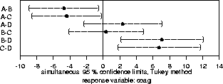
In SPLUS there is a special function multicomp() that handles the details of multiple comparisons. Here are some examples of its use with the coag dataset.

402 > coag.mca _ multicomp(coag.aov,focus="diet")
402 > coag.mca

95 % simultaneous confidence intervals for specified 
linear combinations, by the Tukey method 

critical point: 2.7987 
response variable: coag 

intervals excluding 0 are flagged by '****' 

    Estimate Std.Error Lower Bound Upper Bound      
A-B   -4.710      1.50       -8.90      -0.515 ****
A-C   -4.380      1.50       -8.57      -0.181 ****
A-D    2.370      1.70       -2.38       7.130     
B-C    0.333      1.60       -4.15       4.820     
B-D    7.080      1.79        2.07      12.100 ****
C-D    6.750      1.79        1.74      11.800 ****

402 > plot(coag.mca)

The multicomp() procedure does exactly what is indicated in item #5 above: it tries several methods (including the three mentioned above) of doing multiple comparisons, and then reports to us the best (narrowest intervals) method. You can force it to try a few more computer-intensive methods by saying method="best", or you can force it to use a particular method by specifying the method. Some method choices include:

• method="bon" selects the Bonferroni method.
• method="scheffe" selects Scheffé's method.
• method="tukey" selects the Tukey-Kramer method.
• method="best.fast" selects among several fast methods (including Bonferroni, Scheffé' and Tukey-Kramer); this is the default.
• method="best" also tries some computationally intensive methods in addition to the fast methods, and selects the best (narrowest intervals) result.

402 > multicomp(coag.aov,focus="diet",comparisons="none",
+ method="lsd",error.type="cwe",plot=T)

95 % non-simultaneous confidence intervals for specified 
linear combinations, by the Fisher LSD method 

critical point: 2.086 
response variable: coag 

intervals excluding 0 are flagged by '****' 

  Estimate Std.Error Lower Bound Upper Bound      
A     62.1     0.981        60.1        64.2 ****
B     66.8     1.130        64.5        69.2 ****
C     66.5     1.130        64.1        68.9 ****
D     59.8     1.390        56.9        62.6 ****

Similarly, you could get multicomp() to give the ``uncorrected'' confidence intervals we calculated above when contrasts were introduced, by dropping the ``comparisons="none"'' parameter.

402 > multicomp(coag.aov,focus="diet",method="lsd",error.type="cwe",plot=T)

method="lsd" stands for Fisher's method of least significant differences, which is precisely the unadjusted t intervals we first calculated. Since it has R. A. Fisher's name attached to it, lots of nonstatisticians use it (try searching for `` +Fisher +"least significant difference"'' in Alta-Vista!); however this method does not protect against the degradation of confidence levels in multiple CI's, and it is not much better than the 68%-95%-99% eyeball rule from Statistics 36-201.